Workflow
This release note aims to describe the AIS processing method hosted in the repository (https://github.com/MAPSirbim/AIS_data_processing/tree/v1.0.1), also available at 10.5281/zenodo.4757505. The processing workflow was developed on historical annotated data of the Adriatic Sea (Mediterannean Sea) and aims to (i) identify individual fishing trips and (ii) classify them on a monthly basis according to 5 predefined gear classes: bottom otter trawl (OTB), pelagic pair trawl (PTM), beam trawl (TBB), purse seine (PS), and “other” fishing (OTHER, including dredges and passive gears).
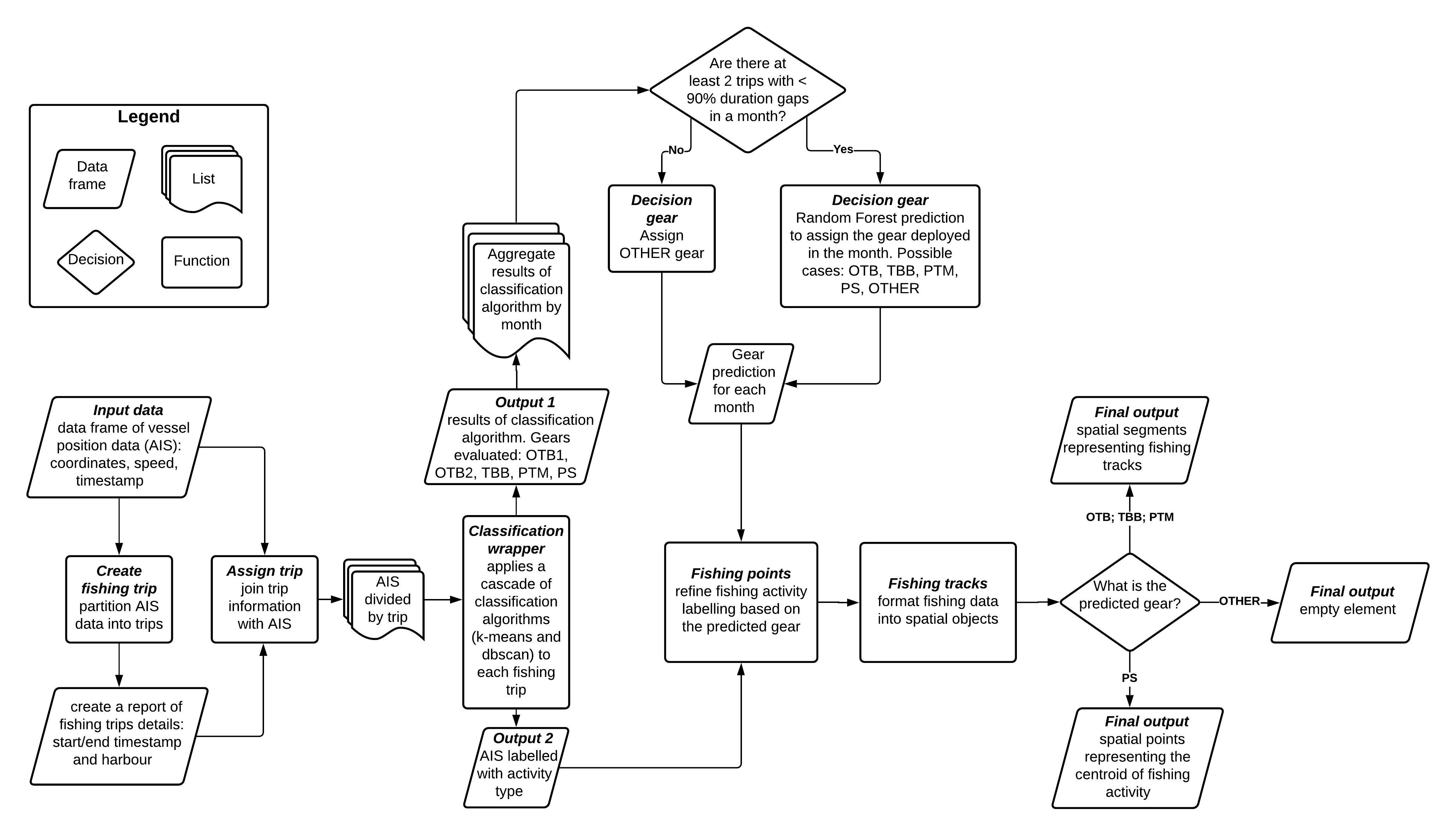
Figure 1: Conceptual framework of the worflow used in AIS data processing
In the repository we also release:
a small subset of AIS signals broadcasted by a few vessels retrieved from the validated dataset (.csv);
- all the parameters required to process the data, such as the input parameters needed to classify fishing trips (.csv) and the trained Random Forest model (.rds) used to finally assign the gear on a monthly basis and finalized to work in the Adriatic Sea;
additional spatial layers required by the data processing (.shp).
Input data
Input data required to start the workflow are described below.
Vessel data
The workflow was originally created to be applied to AIS data. However, it can be adapted to every positioning data type having the following structure:
data = read.csv("data/datatest.csv")
head(data)
## MMSI datetime longitude latitude speed
## 1 1 2015-04-01 17:47:53 13.5027 43.6154 5.3
## 2 1 2015-04-01 17:52:54 13.4914 43.6291 10.2
## 3 1 2015-04-01 17:57:55 13.4914 43.6291 10.2
## 4 1 2015-04-01 18:02:55 13.4952 43.6485 11.0
## 5 1 2015-04-01 18:07:55 13.5068 43.6643 10.3
## 6 1 2015-04-01 18:12:55 13.5175 43.6790 9.5Where:
- MMSI (Maritime Mobile Service Identity): is the unique identifier in official AIS data. For privacy purposes, the MMSI was converted into a fake id (e.g., “1”)
- date and time: timestamp (in the format of Universal Time Coordinate) of broadcasted positions
- latitude and longitude: coordinates of the broadcasted positions (WGS 84)
- speed: instantaneous speed over ground (SOG) of the vessel (kn)
Spatial layers
Three vector layers are required to perform the functions foreseen by the workflow:
- ports (.shp). Port locations were stored as point buffers or manually designed, to best include approach channels to ports, and described by following attributes: name, country and statistical Area (for our scope we use GFCM Geographical Sub-Area; GSA).
- coastal_ban_zone (.shp). Zone where the use of towed gears is prohibited, as defined by Article 13(1) of Regulation (EC) No 1967/2006. It is bounded by 3 nautical miles of the coast or by the 50 m isobath where that depth is reached at a shorter distance from the coast.
- grid (.shp). It is the spatial grid used to aggregate fishing effort and estimate fishing hours. The grid provided in this repository is available here.
These layers cover the Mediterranean basin and should be manually recreated in order to reproduce the processing workflow in different areas.
Processing
The proposed workflow is hereafter applied on a single vessel although it can be iterated on multiple vessels.
vessel = 2
dat = data[which(data$MMSI == vessel),]
head(dat)
## MMSI datetime longitude latitude speed
## 8858 2 2018-06-03 21:41:39 13.5002 43.6224 9.0
## 8859 2 2018-06-03 21:48:44 13.4905 43.6308 5.6
## 8860 2 2018-06-03 21:53:48 13.4836 43.6385 9.0
## 8861 2 2018-06-03 21:56:49 13.4768 43.6463 11.1
## 8862 2 2018-06-03 21:59:51 13.4693 43.6544 11.1
## 8863 2 2018-06-03 22:05:55 13.4540 43.6698 11.1Fishing trip
The create_fishing_trip function identifies vessel-specific fishing trips for each vessel, as sequences of points broadcasted by a vessel, from the time it leaves the port until it returns. To run the function, four datasets are required to complete the entire workflow: the sequence of AIS positions of a vessel, the coastal_ban_zone layer, and 2 layers related to the ports. As AIS transmission gaps (loss of signal of at least 30 minutes) can hamper the identification of the departure and arrival ports, a recovery function was internally applied to join consecutive trips where the departure/arrival port was too far to be assigned. In order to join consecutive trips the function overlays the ending/starting points with the coastal_ban_zone, compares ids between consecutive ending/starting points, compares timestamps and forces a starting and ending port for each trip. In particular, fishing trips are joined and the nearest port is assigned if ending and starting points are consecutive, have a temporal distance shorter than 24 h and at least one is outside the coastal_ban_zone. At the end of the recovery process, for trips that still miss departure and/or arrival ports, the internal function closest_port_recovery is used to force port assignment under other conditions.
dat_trip= create_fishing_trip(data = dat,
                              ports = ports,
                              ports_buffer = port_buf,
                              coastal_ban_zone = coastal_ban_zone)
## ================================================================================
## trip create complete!!!
## Recovery trip
## Recovery harbours================================================================================....complete!!!- data: AIS positions
- ports: port locations (.shp)
- ports_buffer: 1 km buffer, created around the input ports (.shp)
- coastal_ban_zone: zone where the use of towed gears is prohibited (.shp)
The create_fishing_trip function returns the fishing trip table, listing all the trips performed by the vessel and providing information on: departure/arrival timestamps and departure/arrival port names.
head(dat_trip)## MMSI trip start_timestamp end_timestamp departure arrival
## 1 2 1 2018-06-10 21:28:44 2018-06-12 00:04:23 Ancona Ancona
## 2 2 2 2018-06-12 00:16:31 2018-06-14 06:31:33 Ancona Ancona
## 4 2 4 2018-06-17 21:43:24 2018-06-19 00:07:46 Ancona Ancona
## 5 2 5 2018-06-19 00:44:10 2018-06-21 05:04:30 Ancona Ancona
## 6 2 6 2018-06-24 21:36:51 2018-06-26 00:00:42 Ancona Ancona
## 7 2 7 2018-06-26 00:12:50 2018-06-27 00:23:02 Ancona AnconaThe fishing trip table created above is required to assign the fishing trip id to the AIS signals of the vessels. However, the fishing trip table can be useful to store summary information of the fishing trips of a vessel and used to recall records belonging to single trips by using the starting and ending timestamp. In addition, it may be linked with the port layer where information regarding the country and GSA is stored.
The function assign_trip assigns to each AIS position the trip to which it belongs.
dat_with_trip=assign_trip(data=dat,
trip_table=dat_trip)- data: AIS positions
- trip_table: dataframe containing the list of fishing trips and the relative timestamp information (output of the create_fishing_trip function)
The assign_trip function returns the AIS data indexed with trip information
##      MMSI            datetime longitude latitude speed trip
## 9579    2 2018-06-10 21:28:44   13.5021  43.6144   1.7    1
## 9580    2 2018-06-10 21:39:51   13.4925  43.6272   6.8    1
## 9581    2 2018-06-10 21:45:55   13.4860  43.6376   6.7    1
## 9582    2 2018-06-10 21:51:59   13.4827  43.6408   3.0    1
## 9583    2 2018-06-10 21:58:04   13.4750  43.6499  11.0    1
## 9584    2 2018-06-10 21:59:05   13.4750  43.6499  11.0    1
Fishing trip classification and gear assignment
The classification_wrapper function applies a cascade of classification algorithms on each fishing trip, using as input the AIS positions with their assigned trip (dat_with_trip) and the specific parameters needed for each classification algorithm (pars). The classification of each fishing trip is done by two internal functions (classify_speed and search_cluster), whose results are used to label each fishing point according to the speed clusters (in the case of towed gears) or spatial clusters (in the case of PS).
In particular, a k-means algorithms is performed on trip-specific speed values using 5 different sets of centroids that were a priori defined by experts for each fishing gear type (two for OTB, PTM, TBB and PS), the centroids will represent the different speed profiles of fishing behavioural states. The dbscan algorithm is applied on the latitude and longitude data, with two different sets of neighborhood radii (ε) and a number of minimum points in the ε region. The proportions of points falling within each of the identified clusters are used to label the fishing trip as positive or negative to each of the investigated gears.
dat_classified=classification_wrapper(vessel_data=dat_with_trip,
                                      pars=pars,
                                      write.output=T,
                                      output.name = "test1")
## [1] "MMSI: 2 ; start month: 6 ; trip: 1"
## [1] "MMSI: 2 ; start month: 6 ; trip: 2"
## [1] "MMSI: 2 ; start month: 6 ; trip: 4"
## [1] "MMSI: 2 ; start month: 6 ; trip: 5"
## [1] "MMSI: 2 ; start month: 6 ; trip: 6"
## [1] "MMSI: 2 ; start month: 6 ; trip: 7"
## [1] "MMSI: 2 ; start month: 6 ; trip: 9"- dat_with_trip: raw AIS data with an additional column indexing the corresponding fishing trip
- pars: table of parameters required by the classification functions;
- write.output: logical argument to store the data needed to train the Random Forest model.
- output.name: logical argument, specify the name to be given to the output file.
The dat_classified output contains a list with two objects:
- "data_labelled": returns the input data with an additional column for each classification algorithm, indicating the speed cluster assigned by the k-means (in the case of towed gears: otb1, otb2, tbb, ptm) or the spatial cluster assigned by the dbscan (in the case of ps). Clusters 1-2 refer to data gaps or noise, while clusters 3-6 indicate different fishing behavioural states (e.g., hauling, searching, steaming). Besides, a column specifying the month in which the trip started is added.
##       MMSI trip            datetime latitude longitude otb1 ptm tbb ps otb2
## 6.1.1    2    1 2018-06-10 21:28:44  43.6144   13.5021    2   2   2 NA    2
## 6.1.2    2    1 2018-06-10 21:39:51  43.6272   13.4925    2   2   4 NA    2
## 6.1.3    2    1 2018-06-10 21:45:55  43.6376   13.4860    2   2   4 NA    2
## 6.1.4    2    1 2018-06-10 21:51:59  43.6408   13.4827    2   2   2 NA    2
## 6.1.5    2    1 2018-06-10 21:58:04  43.6499   13.4750    2   2   2 NA    2
## 6.1.6    2    1 2018-06-10 21:59:05  43.6499   13.4750    6   6   6 NA    6
##       start_month
## 6.1.1           6
## 6.1.2           6
## 6.1.3           6
## 6.1.4           6
## 6.1.5           6
## 6.1.6 6- "classification_result": contains the binary results of the classification algorithms for each fishing trip and each classification algorithm (otb1, otb2, ptm, tbb, ps); gaps is the percentage (in respect to the duration of the trip) of AIS shutdowns; n_ping is the number of AIS signals belonging to each trip, and start_month is the month in which the fishing trip starts.
##     MMSI trip otb1 otb2 ptm tbb ps       gaps n_ping start_month
## 6.1    2    1    0    0   0   1  0 0.09567679    236           6
## 6.2    2    2    0    0   0   1  0 0.22190249    401           6
## 6.4    2    4    0    0   0   1  0 0.00000000    241           6
## 6.5    2    5    0    0   0   1  0 0.07762446    441           6
## 6.6    2    6    0    0   0   1  0 0.00000000    241           6
## 6.7    2    7    1    1   1   1  0 0.60437641     87           6
In order to accommodate the intra-month variability of the predicted gears, fishing gears are finally reassigned to trips on a monthly basis appling a Random Forest model (RF) using the Random Forest library available in R (Liaw and Viener, 2002). The classification unit of the RF is the set of fishing trips performed in a month by a vessel.
Before training the RF, 524 known vessels (8463 units) are randomly stratified while splitting up into 2 datasets (90:10, dataset 1 and dataset 2, respectively) according to the number of vessels by gear class. The dataset 1 (7572 units) is further splitted in 70:30 equally portioning among the 5 gears (Training and Validation, respectively) to allow model tuning. The dataset 2 (891 units) is used as a test to evaluate classification performance and transferability of the trained RF.
| Gear | Dataset1-vessels | Training-units | Validation-units | Dataset2-vessels | Test-units |
|---|---|---|---|---|---|
| OTB | 282 | 3265 | 1403 | 32 | 516 |
| TBB | 25 | 206 | 91 | 4 | 83 |
| PTM | 36 | 366 | 162 | 5 | 87 |
| PS | 93 | 1119 | 479 | 10 | 149 |
| OTHER | 62 | 342 | 139 | 9 | 56 |
The decision_gear function uses the trained RF to predict the fishing gear for each month. The features used to predict the monthly gear consist in the ratio between the trips labelled as positive for each gear and the total number of the fishing trips (ratio_otb1; ratio_otb2; ratio_ptm; ratio_tbb; ratio_ps).
gear=decision_gear(data=dat_classified[["classification_result"]])- data: requires the binary results of the classification algorithms for each fishing trip (output of the classification wrapper “dat_classified[["classification_result"]]”).
The result of the decision gear function is a summary of the binary results aggregated at monthly level and in addition it gives the output of the RF (i.e., gear).
##   MMSI start_month total_trips valid_trips otb1 otb2 ptm tbb ps ratio_otb1
## 6    2           6           7           7    1    1   1   7  0  0.1428571
##   ratio_otb2 ratio_ptm ratio_tbb ratio_ps gear
## 6  0.1428571 0.1428571         1        0  TBB
Fishing activity
According to the monthly predicted gear, fishing points are identified (identify_fishing_points function) recycling the clusters (k-means - towed gears; dbscan - purse seiners) and retrieving points corresponding to fishing clusters.
fishing_points=identify_fishing_points(data=dat_classified[["data_labelled"]], gear=gear, coord_sys = wgs)- data: requires AIS data, indexed by fishing trip and labelled with the information from k-means and dbscan (output of the classification wrapper “dat_classified[["data_labelled"]]”).
- gear: the result of the decision gear function, containing the gear predicted by the Random Forest classifier
The fishing_point function returns the original AIS data, labelled with the gear identified and with a column (binary) indicating if the points are considered as fishing activity.
## Simple feature collection with 6 features and 5 fields
## geometry type:  POINT
## dimension:      XY
## bbox:           xmin: 13.475 ymin: 43.6144 xmax: 13.5021 ymax: 43.6499
## CRS:            +proj=longlat +datum=WGS84 +no_defs +ellps=WGS84 +towgs84=0,0,0
##         MMSI            datetime trip fishing gear                geometry
## 6.6.1.1    2 2018-06-10 21:28:44    1       0  TBB POINT (13.5021 43.6144)
## 6.6.1.2    2 2018-06-10 21:39:51    1       0  TBB POINT (13.4925 43.6272)
## 6.6.1.3    2 2018-06-10 21:45:55    1       0  TBB  POINT (13.486 43.6376)
## 6.6.1.4    2 2018-06-10 21:51:59    1       0  TBB POINT (13.4827 43.6408)
## 6.6.1.5    2 2018-06-10 21:58:04    1       0  TBB  POINT (13.475 43.6499)
## 6.6.1.6    2 2018-06-10 21:59:05    1       0  TBB  POINT (13.475 43.6499)
The make_fishing_tracks function extracts fishing tracks from fishing points, using a temporal threshold (thr_minute, default value set to 30 minutes) to connect successively ordered fishing points ≤ thr_minutes and avoid false fishing tracks connecting two subsequent fishing events. The result of make_fishing_tracks function is a spatial object where the fishing geometries are stored.
fishing_tracks=make_fishing_tracks(data=fishing_points, coord_sys=wgs, pars=pars)- fishing_points: AIS data labelled with the gear identified and with a column (binary) identifying the data considered as fishing activity
- wgs: coordinate reference system (e.g.: WGS 84)
- pars: object storing the parameter file.
## Simple feature collection with 6 features and 9 fields
## geometry type:  LINESTRING
## dimension:      XY
## bbox:           xmin: 12.8417 ymin: 43.7228 xmax: 13.4016 ymax: 44.0132
## CRS:            +proj=longlat +datum=WGS84 +no_defs +ellps=WGS84 +towgs84=0,0,0
##   MMSI year month gear trip id_track              s_time              f_time
## 1    2 2018     6  TBB    1        2 2018-06-10 22:28:24 2018-06-10 22:59:50
## 2    2 2018     6  TBB    1        4 2018-06-10 23:23:05 2018-06-10 23:47:22
## 3    2 2018     6  TBB    1        6 2018-06-11 00:17:43 2018-06-11 00:48:03
## 4    2 2018     6  TBB    1        8 2018-06-11 01:12:20 2018-06-11 02:01:53
## 5    2 2018     6  TBB    1       10 2018-06-11 02:24:09 2018-06-11 03:01:36
## 6    2 2018     6  TBB    1       12 2018-06-11 03:30:56 2018-06-11 04:07:19
##   range                       geometry
## 1    NA LINESTRING (13.4016 43.7228...
## 2    NA LINESTRING (13.2936 43.7779...
## 3    NA LINESTRING (13.1875 43.836,...
## 4    NA LINESTRING (13.0811 43.9012...
## 5    NA LINESTRING (12.9529 43.9993...
## 6    NA LINESTRING (12.8417 44.0132...
Single command function
The classification_workflow function applies all the functions presented in the previous sections in one single command starting from raw data and returns the fishing tracks/centroids of a vessel. The output type parameter allows storing fishing geometries as points or linestrings.
fishing_tracks=classification_workflow(data=data,
                                       ports=ports,
                                       ports_buffer=port_buf,
                                       coastal_ban_zone = coastal_ban_zone,
                                       pars=pars,
                                       coord_sys=wgs,
output.type="segments")- data: raw AIS data
- ports: .shp of the port locations
- ports_buffer: is the 1 km buffer calculated from the input ports .shp at the beginning of the workflow.
- coastal_ban_zone: .shp of the zone where the use of towed gears is prohibited
- wgs: coordinate reference system (e.g.: WGS 84)
- pars: object storing the parameter file.
- output.type: specify if the output will be the fishing tracks (argument: “tracks”) or the fishing points (argument: “points”).
Estimate fishing effort
Finally, the estimate_fishing_effort function returns a grid populated with cumulative fishing time for the period covered by the input data (hours fishing vessels spent operating gear in each grid cell). Fishing tracks were intersected with the 0.1° grid and durations were computed for each output feature. For towed gears, fishing hours are calculated by dividing resulting lengths by the inherited mean fishing speed. For the purse seiners, fishing hours are calculated by assigning the duration of the cluster to its centroid. The cumulative fishing time was quantified spatial joining each cell with overlapping centroid/portions of hauls, and summing relative durations.
vessel_grid=estimate_fishing_effort(fishing_tracks, grid=grid)- fishing_tracks: spatial object containing the geometries of the fishing activity
- grid: spatial object containing the reticule covering the area of interest that will be intersected with the fishing tracks.
- pars: object storing the parameter file.
head(vessel_grid)## $TBB
## Simple feature collection with 13 features and 5 fields
## geometry type: POLYGON
## dimension: XY
## bbox: xmin: 12.8 ymin: 43.7 xmax: 13.5 ymax: 44.1
## CRS: +proj=longlat +datum=WGS84 +no_defs +ellps=WGS84 +towgs84=0,0,0
## First 10 features:
## grid_id long lat gear f_hours geometry
## 1 26671 13.25 43.75 TBB 12.8032546 POLYGON ((13.2 43.7, 13.2 4...
## 2 26672 13.35 43.75 TBB 11.2467569 POLYGON ((13.3 43.7, 13.3 4...
## 3 26673 13.45 43.75 TBB 0.8733817 POLYGON ((13.4 43.7, 13.4 4...
## 4 26726 13.05 43.85 TBB 3.9796769 POLYGON ((13 43.8, 13 43.9,...
## 5 26727 13.15 43.85 TBB 12.0113021 POLYGON ((13.1 43.8, 13.1 4...
## 6 26728 13.25 43.85 TBB 7.2591725 POLYGON ((13.2 43.8, 13.2 4...
## 7 26778 12.85 43.95 TBB 2.4554332 POLYGON ((12.8 43.9, 12.8 4...
## 8 26779 12.95 43.95 TBB 13.5603859 POLYGON ((12.9 43.9, 12.9 4...
## 9 26780 13.05 43.95 TBB 25.8628391 POLYGON ((13 43.9, 13 44, 1...
## 10 26781 13.15 43.95 TBB 1.2505733 POLYGON ((13.1 43.9, 13.1 4...## Warning in st_centroid.sf(fishing_tracks[[1]]): st_centroid assumes attributes
## are constant over geometries of x## Warning in st_centroid.sfc(st_geometry(x), of_largest_polygon =
## of_largest_polygon): st_centroid does not give correct centroids for longitude/
## latitude data## Simple feature collection with 125 features and 9 fields
## geometry type: POINT
## dimension: XY
## bbox: xmin: 12.86395 ymin: 43.72256 xmax: 13.40083 ymax: 44.05089
## CRS: +proj=longlat +datum=WGS84
## First 10 features:
## MMSI year month gear trip id_track s_time f_time
## 1 2 2018 6 TBB 1 2 2018-06-10 22:28:24 2018-06-10 22:59:50
## 2 2 2018 6 TBB 1 4 2018-06-10 23:23:05 2018-06-10 23:47:22
## 3 2 2018 6 TBB 1 6 2018-06-11 00:17:43 2018-06-11 00:48:03
## 4 2 2018 6 TBB 1 8 2018-06-11 01:12:20 2018-06-11 02:01:53
## 5 2 2018 6 TBB 1 10 2018-06-11 02:24:09 2018-06-11 03:01:36
## 6 2 2018 6 TBB 1 12 2018-06-11 03:30:56 2018-06-11 04:07:19
## 7 2 2018 6 TBB 1 14 2018-06-11 04:25:33 2018-06-11 07:02:16
## 8 2 2018 6 TBB 1 16 2018-06-11 07:30:34 2018-06-11 09:08:38
## 9 2 2018 6 TBB 1 19 2018-06-11 10:32:33 2018-06-11 10:44:41
## 10 2 2018 6 TBB 1 20 2018-06-11 11:21:05 2018-06-11 12:08:36
## range geometry
## 1 NA POINT (13.36876 43.7398)
## 2 NA POINT (13.2686 43.79259)
## 3 NA POINT (13.15581 43.85444)
## 4 NA POINT (13.03584 43.93605)
## 5 NA POINT (12.90643 44.00427)
## 6 NA POINT (12.87636 44.00415)
## 7 NA POINT (12.88186 44.00716)
## 8 NA POINT (12.88271 44.00081)
## 9 NA POINT (12.96613 43.96753)
## 10 NA POINT (12.87543 44.00135)Multiple vessels with different gears
To apply the workflow to multiple vessels and aggregate related fishing activities with different temporal frames (e.g., by year and month), the analysis can be arranged as follow:
- Create fishing segments for all vessels and store them in a list. Each element of the list is a vessel, whose data is again stored in a list as long as the number of different gears predicted for that vessel. The classification_workflow function is applied iteratively on all vessels present in the data and it allows to calculate the fishing geometry in one single command.
all_dat<-read.csv("data/datatest.csv")
all_dat=all_dat[,c("MMSI", "datetime", "longitude", "latitude", "speed")]
all_dat$MMSI=as.character(all_dat$MMSI)
vessels=unique(all_dat$MMSI)
all_fishing_tracks=list()
for(i in 1:length(vessels)){
  cat("\n", "vessel", i, "of", length(vessels))
  cat("\n")
  xvessel=all_dat[which(all_dat$MMSI == vessels[i]),]
  fishing_tracks=classification_workflow(data=xvessel,
                                         ports=ports,
                                         ports_buffer=port_buf,
                                         coastline=coastline,
                                         pars=pars,
                                         coord_sys=wgs,
                                         output.type="segments")
  all_fishing_tracks[[i]]=fishing_tracks
  names(all_fishing_tracks)[i]=vessels[i]
}- Aggregate fishing segments by fishing gear and time period (e.g., month). The first rows of the following code selects all fishing trips that are classified with the same gear. Fishing hours of vessels predicted with the same fishing gear in the same period, are aggregated with respect to a spatial grid to represent the period pattern of spatial activity. In the last rows, grid data is saved in tabular dataframe and in an effort map.
ref_gear=c("OTB", "PTM", "PS", "TBB")

for(j in 1:length(ref_gear)){
  xx=lapply(all_fishing_tracks, function(x){
    rbindlist(lapply(x, function(y){
      if(unique(y$gear) == ref_gear[j]){
        return(y)
      }
    }))
  })
  xgear=ldply(xx, data.frame)
  ref_time=unique(data.frame(xgear)[,c("year", "month")])
  for(i in 1:nrow(ref_time)){
    xvessel=xgear[which(xgear$year == ref_time$year[i] & xgear$month ==   ref_time$month[i]),]
    xvessel_ls=list(xvessel)
    xmap=estimate_fishing_effort(xvessel_ls, grid=grid)
    xmap=ldply(xmap, data.frame)
    xmap$year=ref_time$year[i]
    xmap$month=ref_time$month[i]
    xmap$gear=ref_gear[j]
    xmap=st_sf(xmap)
    saveRDS(xmap, file.path(outdir, "tables", paste0(ref_gear[j], "_", ref_time$year[i], "-", ref_time$month[i], ".rData")))
    worldmap=st_crop(worldmap, st_buffer(xmap, 2.5)) # create map
    xrange = extendrange(xmap$long, f = 1)
    yrange = extendrange(xmap$lat, f = 1)
    xvessel_sf=st_sf(xvessel)
    ggplot()+
      geom_sf(data=worldmap)+
      geom_sf(data=xmap, aes(fill=f_hours), color=NA) +
      geom_sf(data=xvessel_sf, aes(linetype=MMSI, colour=as.factor(trip))) +
      coord_sf(xlim=xrange, ylim=yrange) +
      theme_bw() +
      theme(legend.position = "bottom",
            legend.direction = "horizontal") +
      guides(colour = guide_legend(title = "trip", nrow = 4)) +
      ggtitle(paste0(ref_gear[j], ": ", ref_time$year[i], "-", ref_time$month[i]))
    ggsave(file.path(outdir, "plots", paste0(ref_gear[j], "-", ref_time$year[i], "-", ref_time$month[i], ".png")))
  }
}